Posts are ordered from most recent to least recent.
New Research Reveals Most of the Mass of Star Clusters is Located Outside their Tidal Radius
9 December 2020
Recent research also reinforces the finding that the happenings in star clusters and their respective galaxies are very similar.
Paper Title: EXTENDED STELLAR SYSTEMS IN THE SOLAR NEIGHBORHOOD
Authors: Stefan Meingast, João Alves, and Alena Rottensteiner
First Author’s Institution: Department of Astrophysics, University of Vienna, Türkenschanzstrasse 17, 1180 Wien, Austria
Status: Accepted for Publication in Astronomy & Astrophysics. Open access on arXiv.
In this paper, the authors begin with an explanation of star clusters, the places where stars form, and their importance to galaxies. Later on, the authors also describe how the properties of galaxies that star clusters populate can influence that cluster’s properties.

The photo above depicts the ten clusters that astrophysicists analyzed in this research. Each of the ten was scanned for mass density, radial velocity, and Hertzprung-Russell star distribution, amongst other things.
The research focuses on a finding that determines the important role of global Galactic dynamics in the fate of stellar systems. The results highlight the milky way’s complexity and find a new perspective on the characterization of open clusters.
The early evolution of star systems is not easy to understand because of the “substructured ways in which stars themselves form”, as mentioned in the original paper.
In order to obtain data, the researchers employed several tactics to increase the accuracy of the data, such as limiting parallax.
The member selection procedure is outlined in the next image.

This shows the use of a radial filter and a DBSCAN (will add definitions) in the last row to produce a final culmination of clusters being used in blue.
Hertzsprung-Russell Diagrams for each of the ten clusters that were analyzed are pictured below:

These show a similar shape in the progression of main-sequence stars, a notable occurrence for this research.
After mass measurements and other elements were taken into account, all available figures in the paper itself, the team came up with some conclusions about the stellar clusters.
It was found that nine out of the ten stellar clusters focused on had a cloud around them referred to as the corona.
The stellar populations also had distinct main sequences stars, according to the Hertzprung-Russell Diagrams produced from the cluster analysis. After mass calculations were made, it was discovered that most of the mass in stellar clusters is not part of them internally, but outside in the “corona” around the stellar cluster. The “corona” is a term coined to describe the outer halo that is visible in these star clusters.
Furthermore, each cluster’s rotational pattern reflects the pattern of the Milky Way galaxy as a whole, hinting that the happenings in the galaxy itself highly affect the happenings in individual star clusters. Another factor to consider in this research is that young stars seem to preserve their kinematic properties from birth. More conclusions in the “Conclusions and summary” section of the paper reveal that this research is monumental to a new understanding of stellar clusters in general.
The research’s findings continue to reinforce the fact that the universe continually exhibits new behavior that no one has ever expected before.
~ USAAAO Publicity Team (Kashvi Mundra)
________________________________________________________
Stars with More Metal Composition Attract Smaller Planets, Scientists Determine
14 October 2020
Authors: Cicero X. Lu, Kevin C. Schlaufman, and Sihao Cheng.
First Author’s Institution: Department of Physics and Astronomy, Johns Hopkins University, 3400 N Charles St, Baltimore, MD 21218, USA
Status: Accepted to Astronomical Journal. Open access on arXiv
This article states the potential for small planets to form around dwarf stars. Scientists believe that this potential is likely related to the star’s metallicity.
The forward strides in the planet formation theory have allowed for a type of pebble accretion theory to emerge. However, it is flawed since most of the material in the planetary disk around a young star is lost to the star itself.
The methods used for finding the connection between host star metallicity and small planet occurrence included using logistic regression to “estimate the significance of metallicity and effective temperature for the prediction of planet occurrence”. Then, the team separated the sets into subsamples from which the planet occurrence is calculated independently. Then, with a final mass-radius relation, the team roughly calculated the planet formation efficiency in order to retrieve the data based on planet formation theories.

The diagram shows late dwarf stars as candidates for planet-hosting. The blue dots represent the planet candidate host samples, with the grey being a smoothed-over version of the former.
The occurrence of potential planets is calculated as a function of “orbital period and planet radius in both metal-rich and metal-poor subsamples,” and several computer simulations are employed to create these scenarios, which are described in the paper itself.
A result found in terms of the metallicity of stars was that smaller planets were more likely to form around metal-rich stars. With this strong correlation, the research team concluded that the star’s metallicity plays a big part in determining the occurrence of small planets around a dwarf star.
This occurrence had also been considered in “solar-type stars,” however, the correlation found between their metallicities and the formation of small planets around them was not as strong as it had been for dwarf stars. Since these dwarf stars are much lower in mass than solar-type stars, it can be concluded that these small planets are more common around stars with less mass.
~ USAAAO Publicity Team (Kashvi Mundra)
________________________________________________________
If you’re in search of another Earth-like planet, consider this!
21 September 2020
Paper Title: HABITABLE ZONES IN BINARY STAR SYSTEMS: A ZOOLOGY
Authors: Siegfried Eggl, Nikolaos Georgakarakos, Elke Pilat-Lohinger
First Author’s Institution: Rubin Observatory / Department of Astronomy, University of Washington, Seattle, 98015 WA, USA eggl@uw.edu
Status: Published in MDPI Galaxies. Open access on arXiv.
If you’re trying to look for another planet in the habitable zone of a star, this overview will be quite useful to you. A traditional habitable zone is defined as a region where the temperature is enough so that liquid water can exist near the surface of the planet, and therefore, possibly support life. When considering habitable zones in binary star systems, the amount of energy output from the stars to the planet can vary profoundly, which can prove some otherwise habitable planets as bodies unable to support life. The energy output is known as insolation, which is a clever shortening of the phrase “incoming solar radiation.”
Overview of the Various Habitable Zones
The Isophote based habitable zone relies on a survey of the insolation curves of both stars in the system. As shown in Figures 1 and 2, the habitable zones are not always circular and vary as a result of the stars’ influence on each other. If the stars are of different spectral types, spectral energy distribution must also be taken into account for determining habitable zones.
The main observation is that the Isophote based Habitable Zones of each star seem to be extending outwards towards each other due to the flux of both stars. As the stars are brought closer together, the effect they have on each other’s habitable zone is more pronounced.

“Figure 1: A binary star system with circumstellar habitable zones similar to α Centauri on a compact orbit. The plot shows the system at a distance of ab = 5 au. Single star habitable zones (green) are shown on top of the larger isophote-based habitable zones (red).”

“Figure 2: Same as Figure 1 only for systems with semi-major axes of ab = 3 au and ab = 0.5 au, respectively.”
It turns out that the relation between the distance between the pericenters of two stars and the effect on their habitable zone can be represented in a graph. While the Isophote-based habitable zones technically keep “expanding” from their initial position as the two stars are brought closer together, there is usually a maximum around 10-25% that the zone can extend before orbital instability begins to hover at the outer edge of the habitable zones. This range is for most stars, such as those in the category of our sun and Alpha Centauri.

“Figure 4: A visualization of Equation (19) showing the maximum displacement of the inner (I, dashed) and outer (O, continuous) border of the isophote-based habitable zone as a function of the binary orbit pericenter distance q. The displacement is given in relative to the original single star habitable zone borders. A ∆a = 100% means that the new border is twice as far from its host star than the single star habitable zone pendant. We consider α Centauri-like systems and a binary consisting of two sun-like (G2V) stars.”
While Isophote-based habitable zones are technically habitable zones, planets will not follow the orbits till the outer limits of that zone, or else they will be outside a habitable zone for some time in their orbit around the star. Because of this, radiative habitable zones were introduced by Cuntz (2014) to create a zone where a planet assumed to be orbiting in a circle could reach. This could create an orbit around one star or both stars in the system that a planet is physically capable of reaching and is part of the habitable zone.

“Figure 6: Isophote-based habitable zones and radiative habitable zones for close binary star configurations (P-type). The graphs are for configurations similar to α Centauri only on circular orbits with distances d = 3 au (left panel) and d = 0.5 au (right panel). The inner and outer borders of the single star habitable zone are given by red dashed lines. The red dashed lines in the right panel would represent the habitable zone, if both stars were located at the origin of the graph. The isophote-abscissa intersection points in the left panel are derived from Equations (15) and (16), whereas the ones on the right result from Equation (25), respectively. The radiative habitable zone vanishes for the system in the left panel. The closer system on the right has a radiative habitable zone shown in gray.”
For the systems above, the radiative habitable zones are shown in gray. The first panel’s radiative zone is nonexistent because a planet cannot orbit circularly around the system while also staying in the habitable zone the entire time.
While the habitable zone defined previously (the “traditional” habitable zone) would mean the zone is habitable permanently, there are some instances in which the planet can travel outside the permanent habitable zone if it has a certain so-called “climate inertia”, introduced by Eggl et. al (2012). This would allow for an extension known as the averaged habitable zone that is yet another variable to consider when defining the habitable zones around binary star systems.

“Figure 8 (abridged): Dynamically informed habitable zones around α Centauri A and B. The panels represent a top down view on the actual system. Dynamically stable circumstellar zones around star A and B are colored green.”
What’s The Use?
Overall, the article provides insight into the various types of habitable zones and how habitable worlds are not only present in the traditional, or permanently habitable zone. While Isophote-based habitable zones are the largest and seem the most promising, they are also the most dangerous for this very reason. Extreme caution should be taken with these zones. Aspects such as climate inertia and radiative habitable zones should also be taken into consideration to create a comprehensive report of the habitability status of a planet.
~ USAAAO Publicity Team (Kashvi Mundra)
________________________________________________________
What to Know About the Exoplanet OGLE-2012-BLG-0838Lb
17 September 2020
Title: A Wide Orbit Exoplanet OGLE-2012-BLG-0838Lb
Authors: R. Poleski, B. S. Gaudi, Xiaojia Xie, A. Udalski, J. C. Yee, J. Skowron, M. K. Szymański, I. Soszyński, P. Pietrukowicz, S. Kozlowski, L.Wyrzykowski, K.Ulaczyk, C. Han, Subo Dong, K. M. Morzinski, J. R. Males, L. M. Close, A. Gould, R. W. Pogge, J.-P. Beaulieu, and J.-B. Marquette
First Author’s Institution: Department of Astronomy, Ohio State University, 140 W. 18th Ave., Columbus, OH 43210, USA
Status: Published in the Astronomical Journal of the AAS
Astronomers have recently detected a new exoplanet nearly 13,100 light-years from Earth, but how did they find it and what makes it so special? In this article, we will discuss the techniques used to discover an exoplanet, named OGLE-2012-BLG-0838Lb and what difficulties astronomers faced.
Methods of Detecting Exoplanets:
Because exoplanets are extremely diverse in appearance, temperature, location, and orbital pattern, several different detection techniques can be used to identify them, yet each of them has their own abilities and limitations. The transit photometry method is the most commonly-used way to do this, but is most effective when looking for Kepler exoplanets, which have shorter orbital periods than both gas and ice giants in the Solar System. When looking for smaller planets with wider orbits, the radial-velocity, direct imaging, and microlensing techniques are used, since they are best at detecting these “hot Jupiters”— Jupiter-sized exoplanets with orbital periods less than 10 days. This is because the planets are further away and can be disentangled from the light of the parent star. Also, massive planets cause the parent star to ‘wobble’ more as the center of gravity of the two bodies moves away from the center of the star. Direct imaging is best for detecting planets that are self-luminous, but is not sensitive enough to recognize planets similar in mass to Neptune, approximately 17.15 M⊕.
The technique used to discover OGLE-2012-BLG-0838L is known as microlensing and is successful at uncovering planets kiloparsecs away from us and around low-mass stars. Microlensing is sensitive enough to detect exoplanets that are 1000 times less massive than their parent star and of masses similar to that of Neptune, unlike direct imaging and the previously mentioned techniques.
Observing OGLE-2012-BLG-0838L:
The Optical Gravitational Lensing Experiment (OGLE) aided in the discovery and later observations of OGLE-2012-BLG-0838L. The 1.3-m telescope at Las Campanas Observatory detected a short-lasting anomaly before the main peak of the event, suggesting that its orbit is wide. The planetary nature of that anomaly was later suggested and so, planetary models were fitted. OGLE-2012-BLG-0838 was able to be observed by the EPOXI mission’s Deep Impact spacecraft. However, there were issues with the pictures, since many were out-of-focus, had overlapping figures if taken in the Galactic Bulge, and were donut-shaped, making them difficult to analyze. The Vista Variables in the Via Lactea (VVV Survey) was later used to observe the area around the Galactic Bulge, where the Deep Impact spacecraft could not take clear images, but the VVV survey was not completely successful either. It was able to detect OGLE-2012-BLG-0838, but did not record much useful data.
Shortly after this, the Microlensing Follow Up Network (μFUN) began observing the exoplanet using its ANDICAM dual-beam optical-IR camera at the Cerro Tololo InterAmerican Observatory. Because the observations were completed before the main peak of the anomaly, astronomers were able to see a range of magnifications and get a more accurate measurement for its source flux.
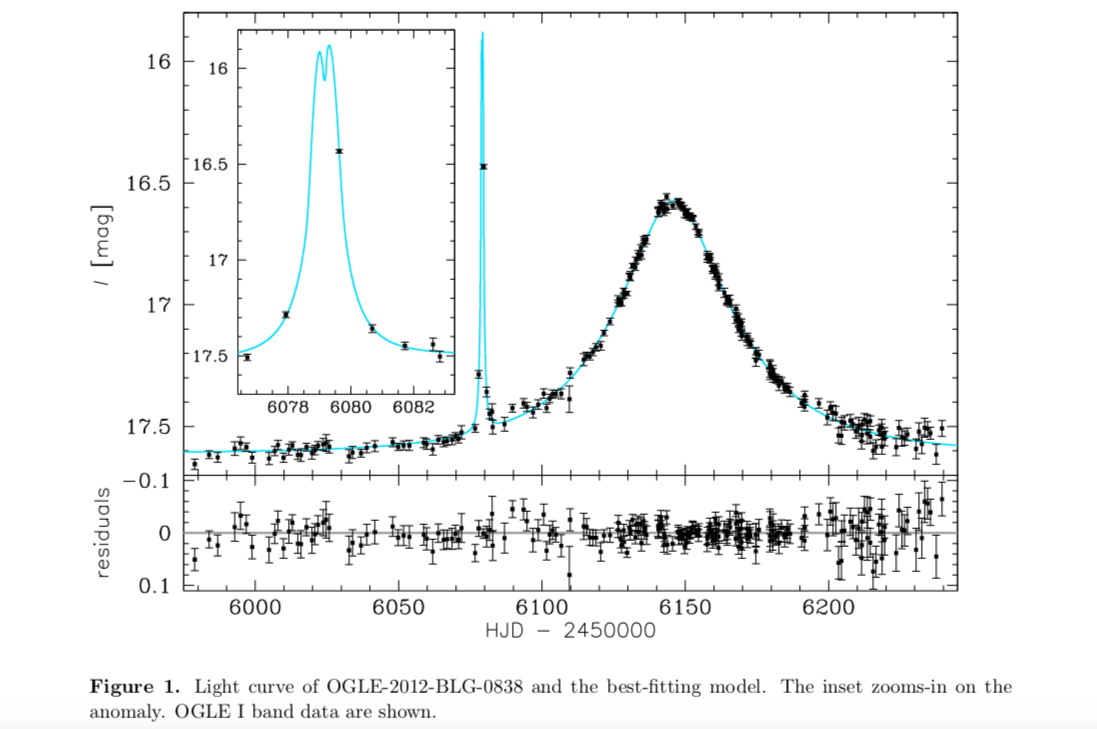
Figure 1. Light curve of OGLE-2012-BLG-0838 and the best-fitting model. The inset zooms-in on the anomaly. OGLE I band data are shown. (Source: Figure 1 from today’s paper)
Models for Microlensing:
By analyzing the light curve above, astronomers were able to see that the anomaly was short and high-amplitude, as evidenced by the height of the curve, but does not have a well determined shape. When an event looks this way, it is either produced by a binary source and a single lens or a single source and a binary lens, and this binary lens can either have a projected separation that is larger or smaller than one. In the case of OGLE-2012-BLG-083, its binary lens has a separation of more than 1, meaning that the graph above is a wide model.
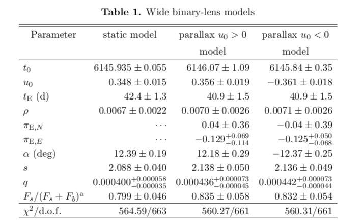
The authors then applied a fitting to the observations allowing them to derive the brightness of the source. Because of deviations in the light curve, astronomers used the lens orbital motion, which determines whether the source motion is linear or not, were used to determine more about the event and its wide binary lens-model. From this, astronomers were able to fit the model.
In conclusion, the discovery and study of OGLE-2012-BLG-0838Lb is particularly fascinating because of the difficulties that astronomers faced. Although pictures of its anomaly were difficult to analyze and initially, not much useful data was recorded, astronomers were still able to learn a bit about the exoplanet.
~ USAAAO Publicity Team (Charly Castillo)
________________________________________________________
Our Sun: The Culprit of Widespread Power Outages
A Culmination of Research
4 September 2020

If you’ve been through a storm, you may have gotten your power knocked out at one point or another. However, how often have you seen total power failure for a major part of a continent? Maybe once in a lifetime, such as the 1989 Quebec power outage.
The culprit of many of these widespread electricity flaws is none other than the same thing that allows life to thrive on Earth — the sun.
The sun is capable of putting out huge ejections of plasma into space, and some of these streams incidentally are detected on Earth. These ejections are called Coronal Mass Ejections, (CMEs), and can have devastating effects on the planet if the conditions are just right.
This type of solar activity was first noticed in 1859 and labeled as a flare related to the geomagnetic disturbances on Earth (Carrington, 1859). The storm had overridden some of the lines in the U. S. telegraph network, and this was the most probable reason why it was noticed. The first clear detection of a CME itself was taken in December of 1971 by Richard Tousey.
In order to understand the mechanics of a CME, we must understand the events happening at the sun. When the magnetic fields on the sun are closed, segments of the outer corona are ejected out into interplanetary space. The closed magnetic fields help the ejections keep their shape and intensity by herding them into a powerful stream that escapes the sun, known as CMEs.
Like anything from the sun, a CME takes time to reach Earth due to the vast distance (93 million miles) between the Earth and the Sun. The amount of time varies with some CMEs taking weeks to reach Earth while others less than a day, according to the SOHO LASCO CME CATALOG (Yashiro et al 2004).
The Advanced Composition Explorer (ACE) studies solar particles and detects a wide range of elements in a CME. Scientists use this device’s data to analyze CMEs and their structure in the data before they reach Earth. Using a particular data value from ACE, the Bz (from ACE Real-Time Solar Wind Data), astronomers have found a distinction to CMEs that are detected. In the beginning, before a CME hits, the data will show a “sheath region”, in which the Bz values will furiously toggle between negative and positive values. Then, when the actual CME hits, the Bz will stabilize in either a positive region or a negative value.
This distinction between the positive and negative values of the Bz is the most important to determining if a geomagnetic storm would’ve hit. If the Bz has a positive value, the CME will not do much. On the other hand, if the Bz has a negative value, then the CME will reconnect with the Earth’s magnetic field and have the potential to cause a geomagnetic storm (Gonzalez & Tsurutani, 1987). This is evidenced by the Bz’s close relation to the DST index (Burton et al 1975), with the DST measuring the disturbance of the magnetic field in the Earth’s atmosphere. Usually, as the Bz starts becoming more and more negative, the DST index will follow suit because of the disturbances in the atmosphere (Burton et al 1975).
In order to obtain more information about the CME, scientists study images (such as H-alpha) and simulations (such as those of JHelioviewer) of the sun to detect magnetic fields and solar filaments on its surface and how they may contribute to the negative-positive Bz orientation of the CME. Solar filaments can have chirality, or north-south orientations, distinguished by their placement in the magnetic fields on the surface of the sun (Martin, 1998). Many studies have indicated that the north-south orientation of a solar filament has a strong correlation with the negative-positive orientation of the Bz for a CME (Yurchyshyn 2001), (Palmerio et al 2018). More research is going on to further solidify this claim.
As such, it is very important to study solar weather not just to advance our scientific knowledge about stars and the sun, but also to detect harmful CMEs from the sun and to potentially avert disaster.
~ USAAAO Publicity Team (Kashvi Mundra)
References
Carrington, R.C., 1859. Description of a Singular Appearance seen in the Sun
on September 1, 1859. Monthly Notices of the Royal Astronomical Society
20, 13–15.
Tousey, R., Brueckner, G. E., Koomen, M. J., & Michels, D. J. 1972, Naval Research
Reviews, 25, 8
Stenzel, R.L. & Gekelman, W. (1981). Magnetic field line
reconnection experiments. 1. Field topologies, J. Geophys.
Res. 86, 649-58.
ACE Mission. (1998). Advanced Composition Explorer (ACE). http://www.srl.caltech.edu/ACE/ace_mission.html
Burton, R. K., R. L. McPherron, and C. T. Russell.: 1975, J. Geophys. Res., 80, 4204.
https://doi.org/10.1029/JA080i031p04204
Martin, S. F. (1998). Filament Chirality: A Link Between Fine-Scale and Global Patterns (Review). In D. F. Webb, B. Schmieder, & D. M. Rust (Eds.), Iau colloq. 167: New perspectives on solar prominences (Vols. ASP Conf. Ser., 150, p. 419).
Yurchyshyn, V. B., Wang, H., Goode, P. R., & Deng, Y.
2001, ApJ, 563, 381
Palmerio, E., Kilpua, E. K. J., Mostl, C., Bothmer, V., James, A. W., Green, L. M., . . .
Harrison, R. A. (2018). Coronal Magnetic Structure of Earthbound CMEs and In Situ
Comparison. Space Weather , 16 , 442-460. doi: 10.1002/2017SW001767
Gonzalez, W. D., & Tsurutani, B. T. 1987, Planetary and
Space Science, 35, 1101 ,
doi: https://doi.org/10.1016/0032-0633(87)90015-8
Yashiro, S., Gopalswamy, N., Michalek, G., St. Cyr, O.C., Plunkett, S.P., Rich, N.B., Howard, R.A., 2004. A catalog of white light coronal mass ejections observed by the SOHO spacecraft. J. of Geophys. Res. 109, A07105.
